Comparing Runtime across Sample Sizes and Number of Taxa • phylobar

Introduction

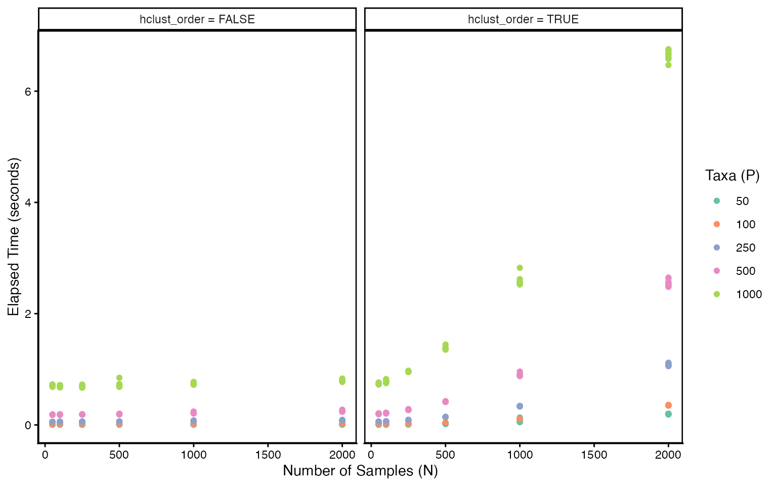
This vignette studies how phylobar’s runtime scales with the number of samples (N) and taxa (P). We simulate random data across a grid of (N, P) values and time each call with system.time(). We also compare runtime with and without ordering samples with hierarchical clustering (the hclust_order argument).

library(ape)
library(ggplot2)
#> Warning: package 'ggplot2' was built under R version 4.5.2
library(phylobar)
theme_set(theme_classic())
set.seed(20260209)

Setup

We simulate one large dataset at the maximum grid dimensions and subset it for each (N, P) combination. This avoids repeated simulation and naming boilerplate inside the timing loops.

n_eval <- c(50, 100, 250, 500, 1000, 2000)
p_eval <- c(50, 100, 250, 500, 1000)
n_reps <- 10

grid <- expand.grid(
    N = n_eval,
    P = p_eval,
    hclust_order = c(TRUE, FALSE),
    rep = seq_len(n_reps)
)

tree_full <- rtree(max(p_eval))
x_full <- matrix(
    rpois(max(n_eval) * max(p_eval), lambda = 5),
    nrow = max(n_eval), ncol = max(p_eval)
)
colnames(x_full) <- tree_full$tip.label
rownames(x_full) <- paste0("s", seq_len(max(n_eval)))

trees <- list()
for (p in p_eval) {
    tips <- tree_full$tip.label[seq_len(p)]
    trees[[as.character(p)]] <- drop.tip(
        tree_full, setdiff(tree_full$tip.label, tips)
    )
}

Timing

For each (N, P, hclust_order) combination we subset the pre-simulated data and time phylobar(). By default phylobar sorts samples using hierarchical clustering, which can be costly when the number of samples is large. It is also often unnecessary when there is already a natural sample ordering (e.g., over time). Setting hclust_order = FALSE keeps samples in their input order.

results <- grid
results$elapsed <- NA

for (i in seq_len(nrow(results))) {
    tree <- trees[[as.character(results$P[i])]]
    x <- x_full[seq_len(results$N[i]), tree$tip.label]

    tm <- system.time(
        phylobar(x, tree, hclust_order = results$hclust_order[i])
    )
    results$elapsed[i] <- tm["elapsed"]
}

Results

results$P <- factor(results$P)
results$hclust_label <- ifelse(
    results$hclust_order,
    "hclust_order = TRUE",
    "hclust_order = FALSE"
)

ggplot(results, aes(N, elapsed, color = P)) +
    geom_point() +
    scale_color_brewer(palette = "Set2") +
    facet_wrap(~ hclust_label) +
    theme(panel.border = element_rect(fill = NA, linewidth = 0.9)) +
    labs(
        x = "Number of Samples (N)",
        y = "Elapsed Time (seconds)",
        color = "Taxa (P)"
    )

Visualization

Here is an example of the phylobar visualization made with $N = 2000$ samples and $P = 1000$ taxa. While phylobar generates the plot SVG elements in a few seconds, the output is both difficult both for the browser to render interactively and for us to visually interperet. We’ve disabled this plot in this documentation because it consumes quite a lot of browser memory drawing all the bars in the barplot.

# very slow rendering, not recommended
phylobar(x, tree, hclust_order = results$hclust_order[i])

In this regime, we recommend using the subset_cluster function to select representative samples to include in the stacked bar plot. Alternatively, separate phylobar views can be made for different sample subsets. As long as we reduce $N$ , we can keep $P = 1000$ and still have smooth interaction.

x_sub <- subset_cluster(x, k = 100)
x_sub <- x_sub[, colSums(x_sub) > 0]
phylobar(x_sub, tree, hclust_order = results$hclust_order[i])

Takeaways

Bypassing the hierarchical clustering step helps in the large $N$ and $P$ setting. When the data are large, it may be worth using a custom, more scalable seriation algorithm to sort the rows of x in advance, and then set hclust_order = FALSE.
While the phylobar function executes quickly, rendering and visual interpretation both suffer when $N$ is large. When $N$ and $P$ are large, the initial view will show $N \times P$ rectangles in the stacked barplot. Rendering all rectangles as SVG elements in the browser can be slow, and stacked bar plots with too many bars are illegible. We recommend either finding representative samples or breaking the exploration into separate subsets of samples.

Session Info

sessionInfo()
#> R version 4.5.1 (2025-06-13)
#> Platform: aarch64-apple-darwin20
#> Running under: macOS Tahoe 26.3
#> 
#> Matrix products: default
#> BLAS:   /Library/Frameworks/R.framework/Versions/4.5-arm64/Resources/lib/libRblas.0.dylib 
#> LAPACK: /Library/Frameworks/R.framework/Versions/4.5-arm64/Resources/lib/libRlapack.dylib;  LAPACK version 3.12.1
#> 
#> locale:
#> [1] C.UTF-8/C.UTF-8/C.UTF-8/C/C.UTF-8/C.UTF-8
#> 
#> time zone: America/Chicago
#> tzcode source: internal
#> 
#> attached base packages:
#> [1] stats     graphics  grDevices utils     datasets  methods   base     
#> 
#> other attached packages:
#> [1] phylobar_0.99.0  ggplot2_4.0.2    ape_5.8-1        BiocStyle_2.36.0
#> 
#> loaded via a namespace (and not attached):
#>  [1] sass_0.4.10         generics_0.1.4      lattice_0.22-9     
#>  [4] digest_0.6.39       magrittr_2.0.4      evaluate_1.0.5     
#>  [7] grid_4.5.1          RColorBrewer_1.1-3  bookdown_0.46      
#> [10] fastmap_1.2.0       jsonlite_2.0.0      Matrix_1.7-4       
#> [13] BiocManager_1.30.27 purrr_1.2.1         scales_1.4.0       
#> [16] codetools_0.2-20    textshaping_1.0.4   jquerylib_0.1.4    
#> [19] cli_3.6.5           rlang_1.1.7         withr_3.0.2        
#> [22] cachem_1.1.0        yaml_2.3.12         otel_0.2.0         
#> [25] tools_4.5.1         parallel_4.5.1      dplyr_1.2.0        
#> [28] fastmatch_1.1-8     vctrs_0.7.1         R6_2.6.1           
#> [31] lifecycle_1.0.5     fs_1.6.6            htmlwidgets_1.6.4  
#> [34] ragg_1.5.0          cluster_2.1.8.2     pkgconfig_2.0.3    
#> [37] desc_1.4.3          pkgdown_2.2.0       bslib_0.10.0       
#> [40] pillar_1.11.1       gtable_0.3.6        glue_1.8.0         
#> [43] phangorn_2.12.1     Rcpp_1.1.1          systemfonts_1.3.1  
#> [46] xfun_0.56           tibble_3.3.1        tidyselect_1.2.1   
#> [49] knitr_1.51          farver_2.1.2        htmltools_0.5.9    
#> [52] nlme_3.1-168        igraph_2.2.1        labeling_0.4.3     
#> [55] rmarkdown_2.30      compiler_4.5.1      quadprog_1.5-8     
#> [58] S7_0.2.1